Perceptron

In this notebook, I will go through how to train a perceptron for binary classification problems.

What is a perceptron?

Perceptron is a artificial neural network whose learning was invented by Frak Rosenblatt in 1957.

According to wikipedia, “In a 1958 press conference organized by the US Navy, Rosenblatt made statements about the perceptron that caused a heated controversy among the fledgling AI community; based on Rosenblatt’s statements, The New York Times reported the perceptron to be “the embryo of an electronic computer that [the Navy] expects will be able to walk, talk, see, write, reproduce itself and be conscious of its existence.”

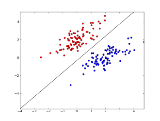
A perceptron is a single-layer, linear classifier:

Although it is very simple (and too simple for many tasks), it forms the basis for more sophisticated networks and algorithms (backpropagation).

A perceptron has $P$ input units, one output unit and $P+1$ weights (parameters) $w_n$. For a particular input (a $P$-dimensional vector ${\bf x}$), the perceptron outputs

$a$ is the activation of the perceptrion. The “sign” function returns $+1$ for anything greater than zero and $-1$ for less than zero.

${\bf w}_0$ is called the “bias weight”. For convenience, we often change the input vector ${\bf x} = (x_1, x_2, …)$ to have $1$ at the end (${\bf x}’ = (x_1, x_2, …, x_p, 1)$), so that we can express the activation as simply $a = {\bf x}’ {\bf w}^\intercal$.

How is a perceptron trained?

In binary classification problems, for each sample ${\bf x}_i$, we have a corresponding label $y_i \in { 1, -1 }$. $1$ corresponds to one class (red points, for example), and $-1$ corresponds to the other class (blue points).

By “training”, I mean that I want to find ${\bf w}$ such that for all $i$, $y_i = sign({\bf x}_i’ {\bf w}^\intercal)$.

In other words, I want to minimize the (0/1) loss function

This is an optimization problem. Unfortunately, this particular loss function is practically impossible to solve, because the gradient is flat everywhere!

Instead, a perceptron learning rule minimizes the perceptron criterion:

• If the prediction was correct - say, $y_i = 1$ and $a = 0.8$, then $-y_i a_i < 0$, so $\max(0, -y_i a_i) = 0$. In other words, the loss is zero for correct examples.
• If the prediction was wrong - say, $y_i = -1$ and $a = 0.8$, then the loss is proportional to $a_i$. The penalty is very large when you predict very large $a_i$ and get it wrong!

It’s important to note that the loss function only cares about the examples that were classified wrong.

So we can also rewrite the loss function as

Now we can take the derivative with respect to ${\bf w}$ and get something nicer:

And, using the stochastic gradient decent algorithm with the learning rate of $\eta$, we get the perceptron weight update rule:

… for all misclassified examples $i$.

(Exercise: take out your papers and pencils and convince yourself of this.)

Training a perceptron

Let’s generate some data X and binary labels y to test on! We’ll use sklearn.datasets to make some test data. Note that we want the targets y to be {-1, 1}.

from sklearn.datasets import make_blobs

X = y = None # Global variables
@interact
def plot_blobs(n_samples=(10, 500),
               center1_x=1.5,
               center1_y=1.5,
               center2_x=-1.5,
               center2_y=-1.5):
    centers=array([[center1_x, center1_y],[center2_x, center2_y]])
    global X, y 
    X, y= make_blobs(n_samples=n_samples, n_features=2,
                      centers=centers, cluster_std=1.0)
    y = y*2 - 1  # To convert to {-1, 1}
    
    plt.scatter(X[:,0], X[:,1], c=y, edgecolor='none')
    plt.xlim([-10,10]); plt.ylim([-10,10]); plt.grid()
    plt.axes().set_aspect('equal')

Exercise 2. implement the code to do a single step of perceptron weight update. Press the button each time to run a single step of update_w_all; re-evaluating the cell resets the weight and starts over.

Remember:

Note that the following code does random train-test split everytime w is updated.

def delta_w_single(w, x, y):
    """Calculates the gradient for w from the single sample x and the target y.
    
        inputs:
            w: 1 x (p+1) vector of current weights.
            x: 1 x p vector representing the single sample.
            y: the target, -1 or 1.
        
        returns:
            w: 1 x (p+1) vector of updated weights.
    """
    # TODO implement this
    return 0

def update_w_all(w, X, y, eta = 0.1):
    """Updates the weight vector for all training examples.

        inputs:
            w: 1 x (p+1) vector of current weights.
            X: N x p vector representing the single sample.
            y: N x 1 vector of the targets, -1 or 1.
            eta: The training rate. Defaults to 0.1.
        
        returns:
            w: 1 x (p+1) vector of updated weights.
    """
    for xi, yi in zip(X, y):
        w += eta * delta_w_single(w, xi, yi) / X.shape[0]
    return w

from numpy.random import random_sample 
w = random_sample(3)   # Initialize w to values from [0, 1)
errors = zeros((0, 2)) # Keeps track of error values over time
interact_manual(perceptron_training, X=fixed(X), y=fixed(y), eta=FloatSlider(min=0.01, max=1.0, value=0.1))

The perceptron only works for linearly separable data.

from sklearn.datasets import make_circles, make_moons
X_circle, y_circle = make_circles(100) # or try make_moons(100)
y_circle = y_circle * 2 - 1
X_circle*=4  # Make it a bit larger
plt.scatter(X_circle[:,0], X_circle[:,1], c=y_circle, edgecolor='none')
plt.xlim([-10,10]); plt.ylim([-10,10]); plt.grid()
plt.axes().set_aspect('equal')

w = random_sample(3)   # Initialize w to values from [0, 1)
errors = zeros((0, 2)) # Keeps track of error values over time
interact_manual(perceptron_training, X=fixed(X_circle), y=fixed(y_circle), eta=fixed(0.1))

As we would have expected, the perceptron fails to converge for this problem.

Download this IPython notebook